Introduction: Low Cost Wireless Sensor Network on 433MHz Band


Many thanks to Teresa Rajba for kindly giving me her acceptance to use data from their publications in this article.
*In the image above - the five sensor-sender units that I used for testing
What are wireless sensor networks?
A simple definition would be: the wireless sensor networks refers to a group of electronic devices distributed on a certain area for monitoring and recording environmental data, that are wirelessly transmitted to a central location to be processed and stored.
Nowadays Wireless Sensor Networks can be used in several ways, bellow are just a few examples:
- Areas of ecological surveillance of forests, rivers, lakes, seas and oceans;
- Possibility to alert in case o terrorist, chemical, biological, epidemic attacks;
- Monitoring systems for children, elderly people, patients or people with special needs;
- Surveillance systems in agriculture and greenhouses;
- Weather-Forecast monitoring system;
- Surveillance of city traffic, schools, car parks;
And many, many other applications.
In this paper I want to show the results of an experiment with wireless sensor networks that have been used for monitoring temperature and humidity data, with a slow and relatively predictable variation. For this experiment I chose to use sensor-senders that I built by my own using affordable modules. The receiver is also DIY, the communication is unidirectional (on the 433 MHz radio band), meaning that the sensors only transmit the data and the central location only receives. There is no communication between sensors and from receiver to sensors.
But why choosing to use multiple transmitters and only one receiver? Obviously the first reason would be “making it simple”. The simpler is the assembling, the less likely it is to fail, and it definitely is much easier to repair and replace the single components in case of malfunctions. Power consumption is also lower, the batteries will last longer (sensors will only consume while monitoring and receiving, the rest of the time the device will be in deep sleep mode). The fact that it is simple makes the device also cheap. Another aspect to keep in mind is the coverage area. Why? It is much easier to build and use a sensitive receiver than to have a sensitive receiver and a powerful transmitter at both the sensors and the central module (this is necessary for a good bidirectional communication). With a sensitive and good-quality receiver it is possible to receive data from a long distance, but emitting data for the same distance requires high emission power and this comes with high costs, electricity consumption and (let’s not forget) the possibility to overrun the legal maximum transmitter power on the 433 MHz band. By using a medium-quality receiver, cheap but with a high-quality antenna (even DIY) and cheap transmitters with a good-quality antenna, we can achieve excellent results at a fraction of the cost of existing wireless sensor networks.
Step 1: Theoretical Considerations
The idea of building a wireless sensor network for monitoring temperature and humidity of air and soil in different areas of a greenhouse came into my mind a long time ago, almost 10 years. I wanted to build a 1-wire network and to use 1-wire temperature and humidity sensors. Unfortunately, 10 years ago humidity sensors were rare and expensive (although temperature sensors were widespread) and since spreading wires all over the greenhouse didn’t seem an option I gave up on the idea pretty quickly.
However, now the situation has radically changed. We are able to find cheap and good-quality sensors (temperature and humidity), and we also have access to cheap transmitters and receivers on the 433 MHz band. There is only one problem: if we have more sensors (let’s say 20) how do we solve the collisions (please keep in mind that this is a one-way communication), meaning, overlapping the emission of 2 or more sensors? While searching for a possible solution I came across this very interesting papers:
Wireless sensor converge cast based on random operations procedure - by RAJBA, T. and RAJBA, S.
and
Basically, the authors show us that the probability of collisions in a wireless sensor network can be calculated if the packets are emitted at certain time points according to a poissonian (exponential) distribution.
An extract from the above paper lists the characteristics of the studied network.
- quite a large number of sensor-sender units N;
- sensor-sender units remain completely independent and switching them on or off is of no influence on network operation;
- all sensor-sender units (or a part of them) may be mobile provided that they are located within the radio range of the receiving station;
- the slowly changing physical parameters are subjected to measurements what means there is no need to transmit the data very frequently ( e.g. every several minutes or several dozens of minutes);
- the transmission is of one-way type, i.e. from the sensor-sender unit up to the receiving point at T average time intervals. Information is transmitted in the protocol at tp duration time;
- any selected sensor starts transmitting randomly at Poisson times. PASTA (Poisson Arrivals See Time Averages) will be used to justify the sending of probes at Poisson epochs;
- all sensor-sender units remain randomly independent and they will transmit the information at a randomly selected moment of time of tp duration and of T average time of repetition;
- if one or more sensors start transmitting while the protocol of tp duration is being transmitted from another sensor, such a situation is called the collision. Collision makes it impossible for central base station to receive the information in a correct way.
It fits almost perfectly with the sensor network I want to test ...
Almost.
I’m not saying that I completely understood the mathematics in the paper, but on the basis of the data presented and on the conclusions I have been able to understand a bit what it is about. The only thing is that a value used in the paper made me worried a little :). It is the variable tp - duration of the data transmission that is assumed to be 3.2x10⁻⁵ s. So the transmission time of the collected data would be 3.2 us! This can not be done on the 433 MHz band. I want to use either the rcswitch or the radiohead to program the transmitter sensors. Studying the codes of the two libraries, I came to the conclusion that the smallest transmission time would be 20ms, well above the value of 3.2 us. With the 2.4 GHz transmitters, it's possible tp time so small… but that's another story.
If we apply the formula proposed by the authors of this paper the result will be:
Initial data( an example):
- Number of sensors N=20;
- Data transmission duration tp=20x10-3 s (0.020s)
- Average transmission interval T=180s
The formula:
Probability of collision on T interval is

if we take into account the initial data the probability of collision on T interval will be 0.043519
This value, which indicates the likelihood of having 4.35 collisions per 100 measurements is, in my opinion, quite good. The probability could improve if we increase the average transmission time, so at a value of 300s we would have a probability of 0.026332, ie 2.6 collisions per 100 measurements. If we consider that we can expect packet data loss anyway during the system's operation (depending on weather conditions for example) then this number is really excellent.
I wanted to do a simulation of this type of network but also a sort of a design assistant, so I made a small program in C, you can find the source code on github (also a compiled binary that is running in windows command line - release).
Input data:
- sensor_number - the number of sensors on the network;
- measurements_number - number of measurements to simulate;
- average_transmission_interval -average time between successive data transmissions;
- transmission_time - the effective duration of data transmission.
Output:
- the calculated maximum measurement time;
- the list of collisions between two sensors;
- number of collisions;
- theoretical probability of the collisions.
The results are quite interesting :)
Enough with the theory, I would not want to insist more on the theoretical part, the articles and the source code are quite eloquent, so I better go to the practical, effective implementation of the wireless sensor network and to the test results .
Step 2: Practical Implementation - the Hardware
For transmitter-sensors we will need the following components:
- ATtiny85 microcontroller 1.11 $;
- Integrated circuit socket 8DIP 0.046 $;
- Temperature/Humidity sensor DHT11 0.74 $;
- 433MHz H34A transmitter module 0.73 $;
- 4xAA battery holder with switch 1$;
Total 3.63 $;
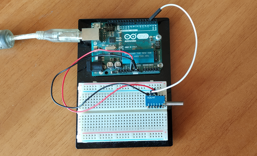
The receiver used for the tests is an Arduino UNO (only for testing) and a H3V4F receiving module (0.66$) with a cheap arc antenna (0.32$).
Sensor-sender schematics

The transmitter-sensor units are powered with 3xAA, 1.5v batteries (in the fourth compartment of the battery holder there is the electronic assembly). As you can see the transmitter’s power supply and the temperature-humidity sensor is hooked to the PB0 pin of the microcontroller (the transmitter and the sensor are powered when the pin is set to HIGH). So when the microcontroller is in deep-sleep mode, it can reach a 4.7uA current consumption. Considering that the wake-up time of the transmitter-sensor would be about 3s (measurement, transmission etc.) and the average time between transmissions of 180s (as the example in the previous chapter), the batteries should resist quite a lot. With some good quality alkaline batteries (i.e. 2000 mAh), autonomy could be over 10 months as calculated on omnicalculator.com (where the total current consumption is: sensor - 1.5mA, transmitter module - 3.5mA and ATtiny85 microcontroller - 5mA, total 10mA).
In the photo below you can see the almost finished sensor-sender assembly.

Below is the photo of the test receiver unit.
Step 3: Practical Implementation - Software
The software uploaded running to the attiny85 microcontroller, the main component of the sensor-sender units, has the purpose to read the data provided by the sensor, convert it to be transmitted by radio, and transmit it within Poisson time frames (exponential distribution or PASTA - Poisson Arrivals See Time Averages). Also, by using a simple function, it monitors the status of the batteries and gives a warning if the required voltage for the sensor is no longer provided. Source code is available on github. The code for the test receiver is very simple I'm posting it below.
//modified rcswitch library from https://github.com/Martin-Laclaustra/rc-switch/tree/protocollessreceiver<br>// the code is a modified version from examples of the original rcswitch library
#include <rcswitch.h>
RCSwitch mySwitch = RCSwitch();
unsigned long data = 0;
void setup() {
  Serial.begin(9600);
  mySwitch.enableReceive(0);  // Receiver on interrupt 0 => that is pin #2
}
void loop() {
  if (mySwitch.available()) {
    unsigned long data = mySwitch.getReceivedValue();
    //output(mySwitch.getReceivedValue(), mySwitch.getReceivedBitlength(), mySwitch.getReceivedDelay(), mySwitch.getReceivedRawdata(),mySwitch.getReceivedProtocol());
    int humidity = bitExtracted(data, 7, 1); //less signifiant 7bits from position 1 - rightmost first bit
    int temperature = bitExtracted(data, 7, 8); // next 7bits from position 8 to the right and so on
    int v_min = bitExtracted(data, 1, 15);
    int packet_id = bitExtracted(data, 3, 16); //3bits - 8 packet id's from 0 to 7
    int sensor_id = bitExtracted(data, 6, 19); //6bit for 64 sensor ID's - total 24 bits  Serial.print(sensor_id);Serial.print(",");Serial.print(packet_id);Serial.print(",");Serial.print(temperature);Serial.print(",");Serial.print(humidity);
    Serial.println();
    mySwitch.resetAvailable();
  }
}
//code from https://www.geeksforgeeks.org/extract-k-bits-given-position-number/
int bitExtracted(unsigned long number, int k, int p)
{
    return (((1 << k) - 1) & (number >> (p - 1)));
}
I've tried to include as many comments as possible to make thing easier to understand.
For debugging I used the softwareserial library and the attiny85 development board with the USBasp programmer(see also my instructable about this). The serial link has been made with Serial to TTL converter(with a PL2303 chip) connected to the bent pins (3 and 4) of the development board (see picture below). All of this has been of an invaluable help to complete the code.

Step 4: Test Results


I have created 5 sensor-sender units that collect and send values measured by the DHT11 sensors. I recorded and saved measurements, with the help of the test receiver and a terminal emulation program (foxterm), during three days. I chose a 48 hour interval for study. I was not necessarily interested in the measured values (sensor 2, for example, it shows me wrong values) but in the number of collisions. In addition, the sensors were placed very close (at 4-5 m) by the receiver to eliminate other causes of packets loss. The test results have been saved in a cvs file and uploaded (look at the file below). I also uploaded an excel file based on this csv file. I took some screenshots to show you how a collision looks like (in my tests of course), I added comments as well to each screenshot.
You may wonder why I did not use a data loader service for example ThingSpeak. The fact is that I have many records, many sensors and data coming often at irregular intervals, and online IoT services only allow data at a certain number of sensors and only at fairly large intervals. I'm thinking in the future to install and configure my own IoT server.
In the end, 4598 measurements on 5 sensor-sender units (aprox. 920/sensor) resulted in a total of 5 collisions for a period of 48 hours (0.5435 collisions/100 measurements). Doing some math (using the wsn_test program with initial data: 5 sensors, average time 180s, transmission time 110 ms) collision probability would be 0.015185 (1.52 collisions/100 measurements). The practical results is even better then the theoretical results isn't it ? :)

Anyway there are also 18 packets lost in this period, so the collisions does not really matter too much in this regard. Of course the test should take place over a longer period of time to get the most conclusive results but in my opinion is a success even in this conditions and fully confirms the theoretical assumptions.

Step 5: Final Thoughts
Immediate application
In a large greenhouse several crops are grown. If the irrigation is manually made with no climate monitoring, without any automation, without data records there is a risk of over or under irrigation and also the water consumption is high, there is no evidence for water consumption optimization, there are risk for crops in general. To avoid this, we can use a wireless sensor network :)
Temperature sensors, air humidity sensors, soil humidity sensors can be placed all around in the greenhouse and with the help of transmitted data several actions can be made: start-stop electric valves for letting the water flow where is needed, start-stop electric fans to reduce temperature in different areas, start-stop heaters as needed and all the data can be archived for future analysis. Also, the system can provide a web interface that is accessible everywhere and email or SMS alarms in case of abnormal condition.
What's next?
- Testing with a larger number of sensors;
- Real-time testing with remote sensors in the coverage area;
- Installing and configuring a local IoT server (on a Raspberry Pi for example);
- Tests also with transmitter(transceiver)-sensors on 2.4Ghz.
so... to be continued... :)
DISCLAIMER : Using the 433MHz frequency band in your region may be subject to radio frequency regulations. Please check your legality before trying this project.

Runner Up in the
Sensors Contest